“A friend is one that knows you as you are, understands where you have been, accepts what you have become, and still, gently allows you to grow.” -William Shakespeare
“Some people go to priests, others to poetry. I go to my friends.” -Virginia Woolf
“There is nothing better than a friend, unless it is a friend with chocolate.” -Linda Grayson
Introduction
Friendship is a significant component of social life in most cultures. Nevertheless, are the friendships behaviours identical among countries? Do the politics, the economy or the geography of a country influence the way friendship is expressed? That is what we will study.
Determining what can foster friendship is a powerful tool to fight the threats of isolation and depression, that are growing each year across the world (especially in “westernized” countries). In some countries, like Japan, a name exists to define a person that completely withdraws from society: Hikikomori (https://en.wikipedia.org/wiki/Hikikomori). In addition to this tendency, the 2020’s sanitary crisis forced many people to isolate themselves. That is why understanding friendship is more crucial than ever.
To do so, we will use data from two social media; from them, we will be able to compute quantitative as well as qualitative friendship characteristics for each country. We will also use datasets with general information about countries and try to explain how they can influence friendship characteristics.
Datasets Presentation
To understand how friendship is expressed, we use two datasets from worldwide social media: Gowalla and BrightKite. Each one of these datasets is composed of two different dataframes. The first one registers all the checkins: who checked in, where and when (see example below). The second one is the friendship relationship between users. Here, undirected friendship are considered (i.e. both have to be friends). Combining the two datasets, we have around 10.9 millions of checkins, 250k users and 1.1 million edges (friendships). Data were collected from Feb. 2009 to Oct. 2010 for Gowalla and from Apr. 2008 to Oct. 2010 for BrightKite.

We also use three datasets that give general information about countries:
- Compilation of UNData: https://www.kaggle.com/sudalairajkumar/undata-country-profiles.
- Compilation of USGovt: https://www.kaggle.com/fernandol/countries-of-the-world.
- happiness2020.pkl and countries_info.csv from “tutorial 01- Handling data”.
We do not enumerate all the characteristics as there are too many, but they encompass a high diversity of themes, like education, economy, healthcare…
Preprocessing
Merging
The merge of the country’s datasets is not trivial. Many issues came from the countries names, that were different depending on the dataset (US or USA). We decided to convert all the country names to the alpha-3 notation that uses three letters to represent each country (however some countries have the same, as best and worst Korea). We also had to remove territories that have a special status and were considered as countries (like Guadeloupe). Eventually, we remained with 127 countries and 40 features for each country.
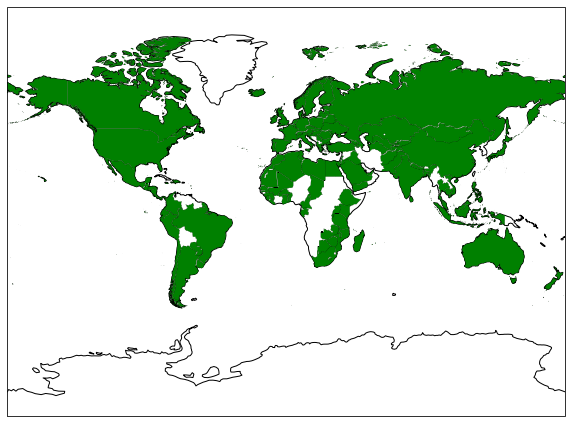 Countries that are present in all the countries facts datasets.
Place of residence
For each user, we computed its place of residence (i.e. its home). We followed the methodology proposed in the paper Friendship and Mobility: User Movements in Location-Based Social Networks, by Eunjoon Cho et al. They propose to discretize the world in squares of 25kmx25km and to compute for each user the square with the most checkins and then, to assign the home as the mean of all the checkins position inside this square. Note that they used the same social network datasets than us. From the home position, we were able to compute the country of residence of each user.
Data reduction
40 features are a lot and not all of them were relevant, so we decided to remove some. In the end, we kept 26 features that may influence friendship. Furthermore, not all countries are good candidates for our study. We have to ensure that the country has enough users and density, so that our results stay relevant.
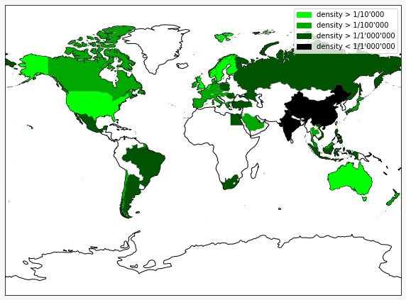 Density of users in each country. Countries in white are not in our dataset.
We see that most of the countries have a minimum density of users and are therefore not relevant. We decided to only keep the country with more than one user per 100’000 inhabitants. Density is not all, in order to study the friendship behaviour we have to ensure that a minimum cluster of people that may be friend exists in the country, so we added a second selection criterion: a minimum of users in the country. It has been fixed to 100. Both the minimum density and the minimum number were found in a heuristic way, trying to maximize them and still have enough countries for an interesting comparison. In the end, we have 47 countries, they are represented below.
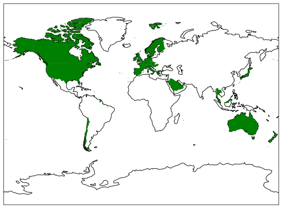 Countries left after all our preprocessing and selection steps.
Friendship characteristics
Computation
Quantitative
First, we are interested in the quantitative aspect of friendship, in the following table we present them:
| Name | Description |
|---|---|
| Nb of friends | The number of friends that the user has |
| Nb of friends in the same country | The number of friends that the user has in the country where she/he lives |
| Ratio of friends in the same country | The number of friends in the same country divided by the total number of friends |
| Nb of friends near | The number of friends that the user has in a radius of 50km around his/her home |
| Ratio of friends near | The number of friends in the vicinity divided by the total number of friends |
Qualitative
We also want to inspect the notion of quality (closeness). To do so we use the following features:
| Name | Description |
|---|---|
| Avg nb of meeting | The number of times that a user meets her/his friends |
| Nb of meeting with his/her best friend | The number of meeting that the user had with her/his best friend |
| Nb of friends met | The number of friends that the user has met at least one time |
We consider that two users met if they checked in the same place within a 30min interval. The best friend is the friend that the user has met the most. The best friend information has been created because most of the friends never met, as a consequence the distribution of meetings is hard to deal with. We hope that the number of meetings with the best friend may represent in a better way the meeting interaction between friends.
Compute and merge
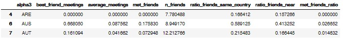
For each user, we compute her/his characteristics:

Then, we regroup all the user’s information with respect to their countries, and we compute the mean of each feature for each country. Note that, when available, we only keep the ratio and not raw numbers.
Inspection
Now that we have computed the friendship characteristics, we can inspect them to see if the features vary depending on the country.
Clustering
One first and naive way is to perform clustering on the friendship features of each country to see if some countries share similar behaviours (data have been standardized before). We use Gaussian Mixture Model for the clustering, as it provides more flexibility than K-means that assumes spherical clusters. We compute the merge for a number of clusters varying from one to the total number of countries and evaluate the AIC and BIC metrics. These metrics have to be minimized; their results are plotted below as well as the cluster assignment.
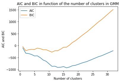 AIC and BIC values for GMM clustersing of the friendship features with respect to the number of clusters.
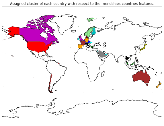 Clusters resulting of a GMM clustersing of the friendship features with 12 clusters.
The optimal number of clusters is around 12 clusters, which indicates that the friendships characteristics vary among countries. If the features would have been similar within some groups of countries the number would be smaller. That is what happened for the same cluster method applied to the countries features, the optimal number of clusters was 4. That ensure that it exists some common relations, one can find their cluster assignment below. Interestingly, Northern, Central and Southern Europe are quite well clustered. The importance of the economy in the general country features may explain this separation.
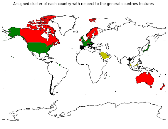 Clusters resulting of a GMM clustering of the countries facts with 4 clusters.
PCA
Another way to see that the features vary across countries is to use the loadings of the Principal Component Analysis (PCA). First, we apply a standard PCA on the whole information about countries (friendship means and general facts) and we find the principal components (PC), for each PC, we can compute its loadings (how much each initial feature influenced it). The PCs that explain 95% of the variance have the following principal initial features: health expenditure, energy supply per capita, happiness score, age distribution, individuals using Internet, number of friends, urban population, tertiary education, GPD growth rate, coastline, GPD per capita and average meetings. It is interesting to see that among the features that explain 95% of the variance two information are related to friendship, which means that it is not constant among countries.
Boxplots
A more robust way to analyze the data is to plot the boxplot of each feature among the countries and compare them.
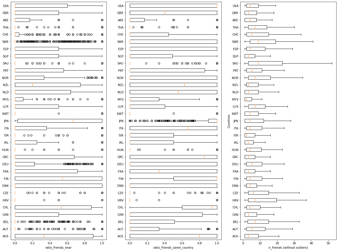 Boxplots of the quantitative features in each country.
Let’s start with the quantitative features (above). First, for the ratio of near friends, we see entirely different results depending on the country. Some boxplot embrace the whole range of possibilities, and others are concentrated around zero with some outliers. The behaviour may depend on the country density of population and other factors. Second, for the ratio of friends in the same country, some different values appear. The most striking one is Japan that, in opposition to a lot of countries, have residents who are mainly friends with other Japanese. Some cultural and geographical reasons may explain this. The distribution of the number of friends is more similar between the different countries, although not identical. Please note that for this last plot we do not show the outliers because some of them have very high values and so the distribution is hard to see.
Quantitative friendships characteristics definitely seem to be influenced by the country.
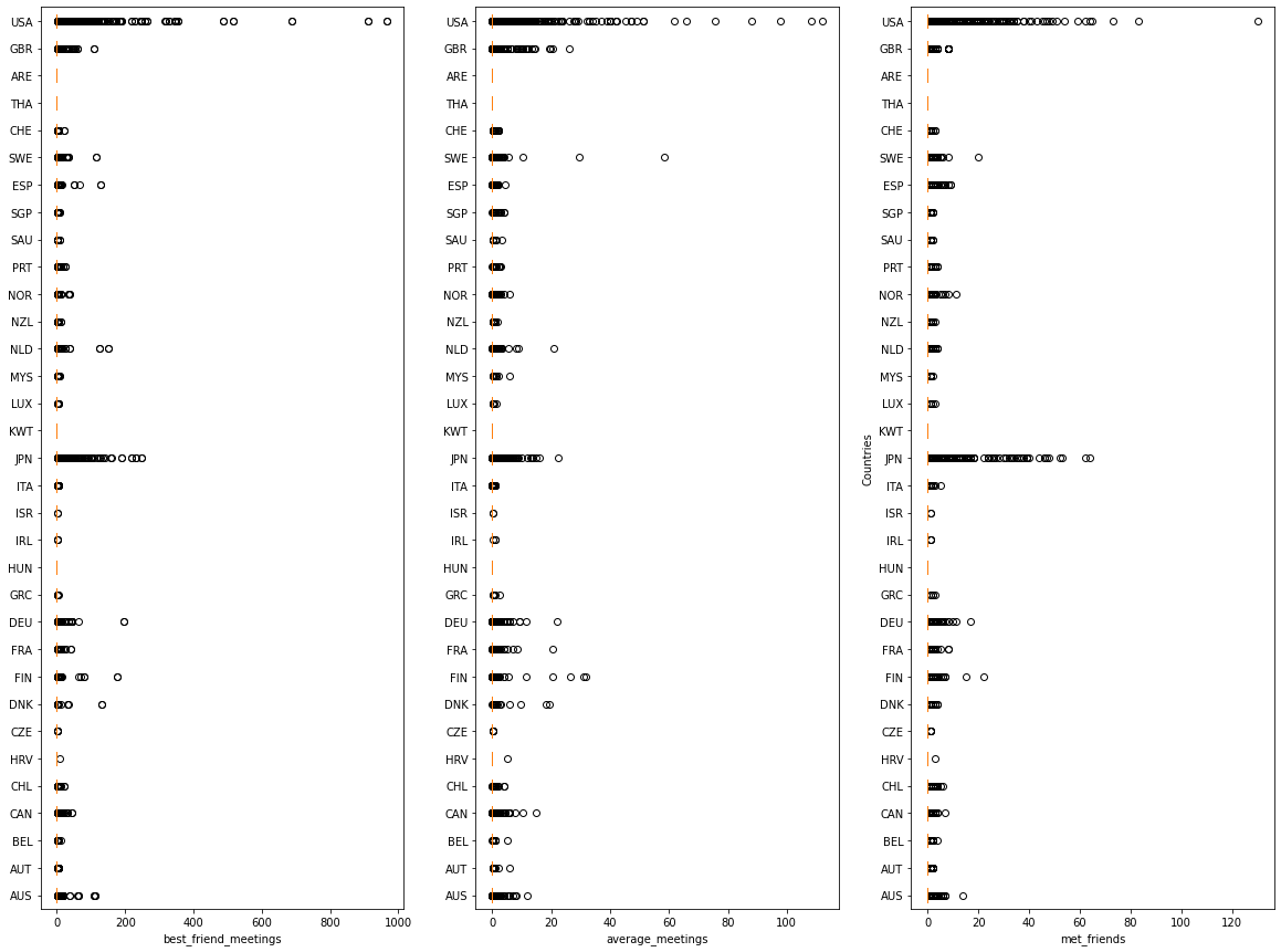 Boxplots of the qualitative features in each country.
Now, we can have a glance at the qualitative features. We see that for all the countries and all the features, the distribution is close by zero. This is due to the fact that most of the users never met their friends. As a consequence, it hard to say if there is a difference between the countries from this plot.
Qualitative friendships characteristics have a lot of zero values.
Statistical tests
We saw that some features seem to have differences among countries, we want to verify that in a statistical way.
One-way ANOVA test
One-way ANOVA (ANalysis Of the VAriance) is one way to do it. The null hypothesis of this method assumes that samples in all groups are generated by populations with the same mean and that all distributions are normal. If we refute the null hypothesis, it means that at least one population is generated by a different mean. Here our samples are the values of the friendship characteristic, and the groups are the country. In the following table, we present the results for the One-way ANOVA tests:
| Feature | P-value |
|---|---|
| Nb of friends | 0 |
| ratio of friends in the same country | 0 |
| ratio of friends near | <0.01 |
| Avg nb of meeting | <0.01 |
| Nb of meeting with his/her best friend | <0.01 |
| Nb of friends met | <0.01 |
With such low p-values we can reject the null hypothesis for all the features. That means that at least one of the group (country) has been generated by a distribution that has not the same mean as the others.
However, these results have to be considered with precautions as it is not sure if the normal distribution condition is satisfied. For example, if we plot the histogram of the average meetings in Canada, we see that the distribution is more similar to a power-law than to a Gaussian, same happens with some of the countries.
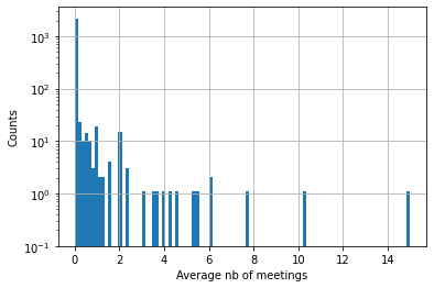 Histogram of the average number of meetings in Canada.
Kruskal-Wallis test
To handle this issue, we can use the Kruskal-Wallis test that does not assume a normal distribution. This time, the null hypothesis is that the median of each group is the same. The computation gives us:
| Feature | P-value |
|---|---|
| Nb of friends | 0 |
| ratio of friends in the same country | 0 |
| ratio of friends near | 0 |
| Avg nb of meeting | < 0.001 |
| Nb of meeting with his/her best friend | < 0.001 |
| Nb of friends met | < 0.001 |
Again, we can refute the null hypothesis; as a consequence, the samples of at least one group have been generated by a distribution that does not have the same median as the others.
Statistical tests proved that friendship features vary across countries.
Relation between countries and friendship features
We know that the country of residence impacts friendship behaviours. We will try to figure out, with the country facts dataset, if we can infer what are the differences between countries that are responsible for how friendship is expressed.
Correlation matrix
Let’s take a glance to the correlation matrix to see which features may be correlated. We will highlight the different correlation that may make sense and that have at least 0.3 value of correlation.
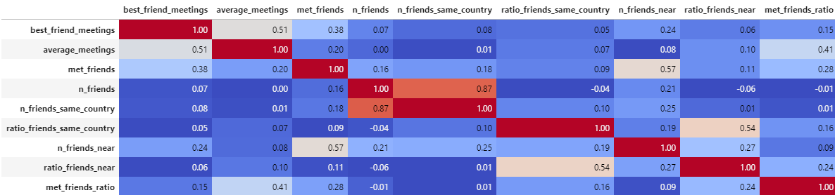
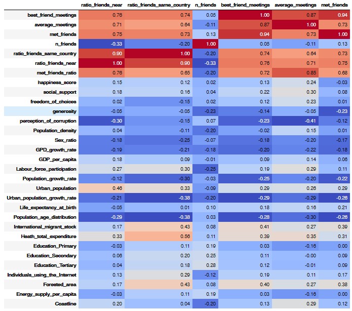 Correlation matrix of the friendship features with all the features.
Intercorrelation between the friendship features:
- The three qualitative features are highly correlated, which makes sense as someone who is used to meet his friend will have more meetings and meet more often his/her best friend.
- The ratio of near friends and friends in the same country is correlated, which is logical.
- The qualitative characteristics depend on the number of friends near and in the same country. We explain that by the fact that it is easier to meet someone near.
The ratio of friends near to the user seem to be influenced by urban population: if a country has more urban population, people will have friends that live closer.
The ratio of friends in the same country also seems to be correlated to urban population: people in the cities may have more access to Internet, and so are more able to be friends with compatriots. However, the urban population growth rate has the opposite effect and may hide a hidden feature.
The number of friends doesn’t seem to be influenced by the countries features.
The three qualitative features show some correlations but there is no explanation for them.
Friendship features are highly intercorrelated and some of them are correlated to some countries features.
Regression
In the last section, we highlighted some correlation, but the value of correlation is not sufficient. It is also necessary to see to which extent we can trust the result. That it is why we apply a regression from all the countries features to each friendship characteristic, note that, before regression, data are standardized.
In the following tables we will show for each friendship feature what country feature influences it with more than 0.05 of p-value.
Ratio of friends near
| Feature | Coef | P-value |
|---|---|---|
| Generosity | -1.04 | 0.02 |
| Perception of corruption | -1.63 | 0.03 |
| Primary Eudcation | -404.79 | 0.03 |
| Energy supply per capita | 407.80 | 0.03 |
Ratio of friends in the same country
| Feature | Coef | P-value |
|---|---|---|
| Generosity | -0.82 | 0.033 |
| Perception of corruption | -1.27 | 0.04 |
Total number of friends
For this regression a lot of features have a low p-value, we only display the ones that have a logical explanation.
| Feature | Coef | P-value |
|---|---|---|
| Forested area | -59.96 | 0.03 |
| Tertiary Education | 0.49 | 0.05 |
| Primary Eudcation | 446.79 | 0.01 |
| Urban population | 0.76 | 0.02 |
| GDP per capita | 0.96 | 0.01 |
Average number of meetings
No feature has less than 0.05 of p-value
Number of friends met
| Feature | Coef | P-value |
|---|---|---|
| Perception of corruption | -1.87 | 0.03 |
Number of best friends meetings
| Feature | Coef | P-value |
|---|---|---|
| International migrant stock | 90.97 | 0.01 |
| Forested area | -90.35 | 0.01 |
Discuss the regression
A lot of these results make no sense, for example, that the generosity diminishes the number of friends near. They are the results of hidden features. That will be discussed in the chapter “Discussion”.
However, some of the relations are interesting and make sense. The inverse correlation between the number of friends and the forested areas, for example, as high forested countries may be less suitable to travel and to highly dense areas.
Using regression, we can find some interesting relation between country features and friendship expression. But, we also see relations due to hidden features.
Pairplot
One may argue that we did not find good relations during the regression because we are doing linear regression. However, a glance at the pairplots shows that most of the paired comparison are random, and sometimes have some linear tendency.
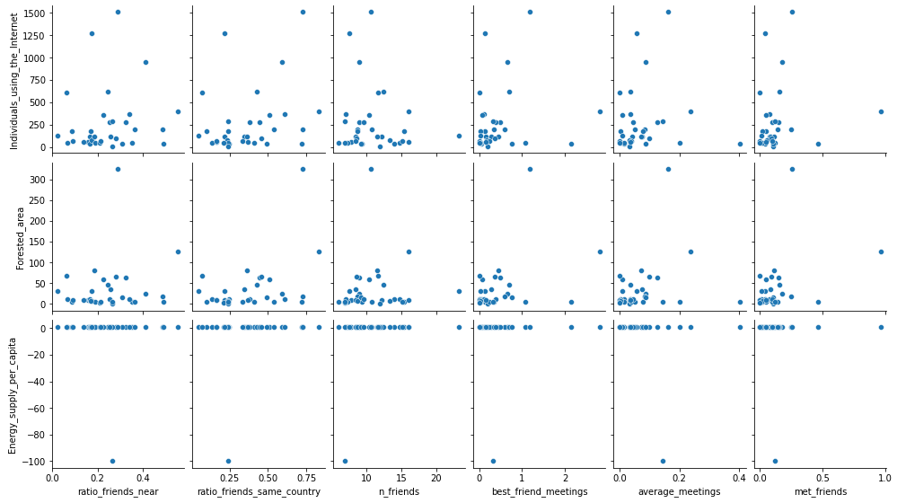 Extract of the pairplot of the friendship features with all the features.
Relation between quantitative and qualitative friendships characteristics
Correlation matrix
Let’s take a look at the correlation matrix to analyse how the friendship characteristics affect each other.
 Correlation matrix of the friendship features between them.
We can see some logical results:
The more near friends you have the more you meet friends.
Of course, the more friends you have near the more friends you have in the same country.
The more meetings you have with friends on average the more you see your best friend.
As a conclusion:
So, if you want to make strong frienships meet your friends more often. And if you want to meet your friends more often, take care of those friends who live near.
Regression
The results of the regressions computed are not representative as the R-squared scores are:
| Feature | R-squares |
|---|---|
| best_friend_meetings | 0.058 |
| average_meetings | 0.014 |
| met_friends | 0.327 |
| met_friends_ratio | 0.058 |
In this case p-values were acceptable for most features but as the R-squared are so low we conclude that on friendship feature cannot be explained by the other features. Demystifying somehow the rumors that those who have a lot of friends do not have good friends.
Relation between happiness and friendship
Correlation matrix
Let’s take a look at the correlation matrix to analyse how the friendship characteristics affect each other.
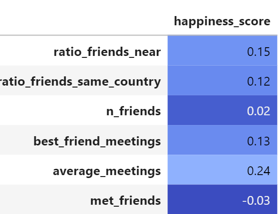 Correlation matrix of the friendship features between them.
The friendship characteristic the most related to the happiness is the average number of meetings.
This leads us to think that it does not make one happy to have a lot of friends but to really connect with them. That is why in these times of pandemic we need to really take care of those close friends with whom we can connect in real life (always with security protocols).
Regression
The results of the regressions computed are not representative as the R-squared score is 0.307. Maybe if we had the happiness score of each user we could exploit the whole users’ dataset to see if there is any relation.
Discussion
Clustering, Boxplots, PCA and Statistcal Tests all suggest that friendship characteristics vary across countries. The most meaningful way to adress this, is the KW-statistical test; however it only allows to conclude that at least one country shows significantly different friendship behaviors. The other methods are not as rigorous, but suggest that many contries are different in terms of friendship.
Quantitative friendship characteristics seem to be correlated with coutry features, as the regressions showed high R-squared scores and low p-values for some country features. However, our study fails to determine if there is a causality link between those features; we can only make hypothesis based on common sense. Some correlations are not really intuitive and may be caused by hidden features. As a matter of fact, the perception of corruption is correlated with quantitative friendship characteristics, but it is probably more the democratization and freedom that affects both the perception of corruption and the access to social media, hence the quantity of friends in Gowalla and Brightkite.
On the other hand, qualitative friendship characteristics were not found to be correlated to any country features. Interestingly, we realized that most of the friends actually never meet, which explains why not much can be said about qualitative characteristics based on the available data. Furthermore, this fact questions whether Gowalla and Brightkite really encompass representative friendship characteristics: people are mostly friends with people they never met. Moreover the data might correspond mostly to one specific category of people (acces to interent, acces to smartphone or computer, most of the users are Americans, etc.).
The fact that the Gowalla and Brightkite users might not be representative of the overall friendship relations could explain why we did not find any link between friendship and happiness, nor between qualitative and quantitative friendship metrics.
Finally, if we could restart the project from the beginning, we would review some of our choices. First, we would select other datasets than the ones that we used. A social media with more users and more widespread would be easy to find nowadays. Secondly, we would include other features in the general fact dataset, especially cultural features that were missing here and maybe have more influence.
Conclusion
In this report we were interested in studying the influence of the place of residence of a user on how she/he expresses her/his friendship. To do so we used five different datasets. Two came from social media and provided us the friendships relations as well as the checkins done by the users at different times and places. The three others datasets were composed of general information about countries.
Based on the social media dataset we computed for each user its place of residence, some quantitative and qualitatives friendship metrics. The inspection of this information exhibited the diversity of type of friendshipy depending on the country. This was also confirmed by statistical tests.
Then, we tried to understand the causes of these differences by looking at the correlation matrix and trying to do a regression from country features to friendship features. For the quantitative features, it was possible to find some interesting relations. However, for the qualitative ones no relation could be found. This is mainly due to the fact that users meet rarely. For both qualitative and quantitative features, some of the relations where hidding other features.
In parallel, we tried to understand if there was a link between quantitative and qualitative friendship features. However, we were unable to find one. Furthermore we were unable as well to find strong relations between happiness and friendship chracteristics.
The main reason of our difficulties to infer results is the size of the dataset and how the people behave in it. The number of users is huge, however distributed along the world it is not that impressive. So, it was hard to correctly and precisely capture the countries behaviour. People on a social media don’t necessarily behave as people on real life, especially, in this case they rarely met, which critically impacted our measure of the quality of friendship.
Eventually, we were able to show that friendship is not expressed in the same fashion everywhere, but we were only able to predict poorly what makes that residents of a country express friendship in a certain way. Nevertheless, we can advise States to improve their means of transport: we don’t think that people living in forest or in rural areas have less friends, but it harder for them to meet. We can also advise to invest in education - not saying that educated people are more friendly - but that they are able to find more stable job and so to meet they friends more often.